Introduction to Random Variables
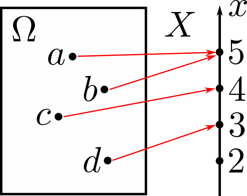
A random variable \(X\) is a function or a mapping from the sample space \(\Omega\) to the real numbers, i.e., it associates a real number to every possible outcome. Mathematically, we say that
\[X:\Omega\rightarrow\mathbb{R}.\]We denote a random variable by a capital letter, e.g., \(X\), and its numerical values by a small letter, e.g., \(x\). A function of one or several random variables is also a random variable. For example, \(X+Y\) is a random variable whose value is \(x+y\) when \(X=x\) and \(Y=y\). There can be several random variables defined on a single sample space.
A random variable can be discrete or continuous. Consider tossing a coin 5 times. We can define a random variable as the number of heads that come up. In this case, we have a discrete random variable. We might also consider the height of students in a university, in which case we have a continuous random variable. In this section, we will be dealing with discrete random variables.
Discrete Random Variables
A discrete random variable takes countably many values. We say that a set is countable if we can put the elements into a one-to-one correspondence with the set of integers.
Probability Mass Function (PMF)
The probability mass function \(p_X(x)\) of a discrete random variable \(X\) is its probability law or probability distribution. It is the probability that \(X\) will take the value \(x\), i.e.,
\[p_X(x)=\mathbf{P}(X=x)=\mathbf{P}(\{\omega\in\Omega:X(\omega)=x\}).\]Example
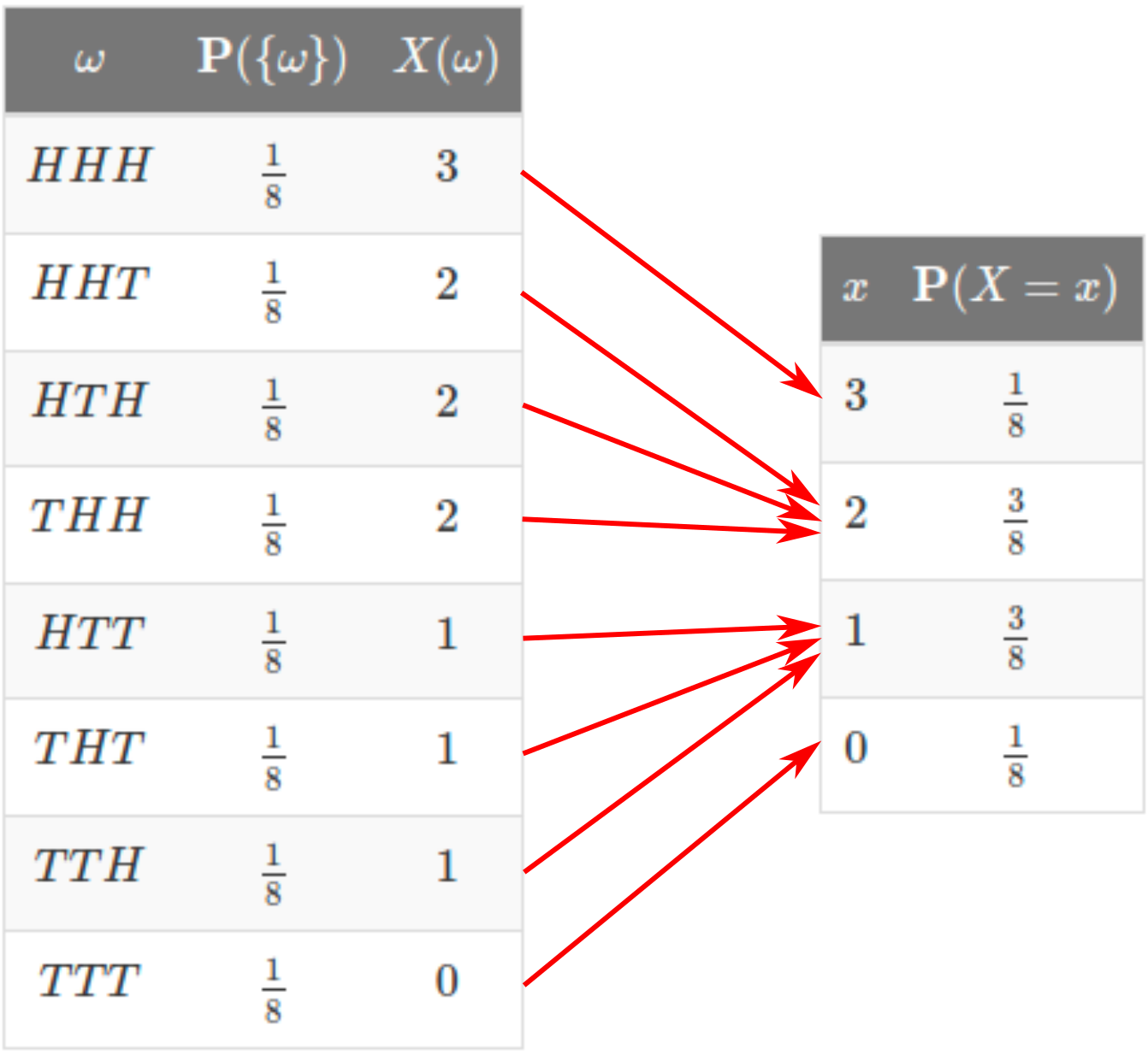
Consider tossing a fair coin 3 times and define the random variable \(X\) as the number of heads. We summarize all the possible outcomes of the experiment on the left table below. To extract the PMF, we add the probabilities of outcomes with the same number of heads. These are summarized on the right table.
Expectation
The expectation or mean of a discrete random variable is defined as
\[\mathbb{E}[X]=\sum_{x}xp_X(x).\]Properties of Expectations
- If \(X\geq0\), then \(\mathbb{E}[X]\geq0\).
- If \(a\leq X\leq b\), then \(a\leq\mathbb{E}[X]\leq b\).
- If \(c\) is a constant, then \(\mathbb{E}[c]=c\).
-
Expectation of \(g(X)\)
\[\mathbb{E}[g(X)]=\sum_{x}g(x)p_X(x)\]Warning: In general, \(\mathbb{E}\!\left[g(X)\right]\neq g\left(\mathbb{E}[X]\right)\). -
Linearity
\[\mathbb{E}[aX+b]=a\,\mathbb{E}[X]+b\]
Variance
The variance is a measure of the spread of a probability mass function. If \(X\) is a random variable with expectation \(\mathbb{E}[X]=\mu\), then its variance is defined by
\[\mathrm{var}(X)=\mathbb{E}\!\left[\left(X-\mu\right)^2\right].\]The variance is always positive or zero, i.e., \(\mathrm{var}(X)\geq0\). A random variable whose
From the variance, we can calculate the standard deviation \(\sigma_X\) of a random variable:
\[\sigma_X=\sqrt{\mathrm{var}(X)}.\]Properties of the Variance
-
The variance of a linear function of \(X\) is
\[\mathrm{var}(aX+b)=a^2\mathrm{var}(X).\]Proof:$$\begin{align} \mathrm{var}(aX+b)&=\mathbb{E}\!\left[\left(aX+b-\mathbb{E}[aX+b]\right)^2\right]\\ &=\mathbb{E}\!\left[(aX+b-a\,\mathbb{E}[X]-b)^2\right]\\ &=\mathbb{E}\!\left[a^2(X-\mathbb{E}[X])^2\right]\\ &=a^2\,\mathbb{E}[(X-\mathbb{E}[X])^2]\\ &=a^2\mathrm{var}(X) \end{align}$$
-
A useful formula for variance is
\[\mathrm{var}(X)=\mathbb{E}[X^2]-\left(\mathbb{E}[X]\right)^2.\]Proof:$$\begin{align} \mathrm{var}(X)&=\mathbb{E}[(X-\mu)^2]\\ &=\mathbb{E}[X^2-2\mu X+\mu^2]\\ &=\mathbb{E}[X^2]-2\mu\,\mathbb{E}[X]+\mu^2\\ &=\mathbb{E}[X^2]-2(\mathbb{E}[X])^2+(\mathbb{E}[X])^2\\ &=\mathbb{E}[X^2]-(\mathbb{E}[X])^2 \end{align}$$