Binomial Distribution | The Science of Data

Consider $n$ independent trials where the outcome of each trial is either a success with probability $p$, or a failure with probability $1-p$. The number of successes in $n$ independent trials is described by a binomial distribution with two parameters $n$ and $p$. We denote it by $\mathrm{Binom}(n,p)$.

Probability Mass Function

The probability mass function of a binomial distribution is given by

\[p_X(k)=\binom{n}{k}p^k(1-p)^{n-k}\]

where $k=0,1,2,\ldots,n.$

Expectation

The expectation of a binomial distribution is

\[\mathbb{E}[X]=np.\]

Proof:

$$\begin{align} \mathbb{E}[X]&=\sum_{k=0}^{n}k\binom{n}{k}p^k(1-p)^{n-k}\\ &=\sum_{k=1}^{n}k\,\dfrac{n!}{k!(n-k)!}p^k(1-p)^{n-k}\\ &=\sum_{k=1}^{n}\dfrac{n!}{(k-1)!(n-k)!}p^k(1-p)^{n-k}\\ &=np\sum_{k=1}^{n}\dfrac{(n-1)!}{(k-1)!(n-k)!}p^{k-1}(1-p)^{n-k}. \end{align}$$ We let $$k=j+1$$ so that $$\mathbb{E}[X]=np\sum_{j=0}^{n-1}\dfrac{(n-1)!}{j!(n-1-j)!}p^j(1-p)^{n-1-j}.$$ Now, from the binomial expansion formula, we have $$(a+b)^{n-1}=\sum_{i=0}^{n-1}\dfrac{(n-1)!}{i!(n-1-i)!}\,a^{i}b^{n-1-i}$$ so that $$\begin{align} \mathbb{E}[X]&=np\left[p+(1-p)\right]^{n-1}\\ &=np. \end{align}$$

Simpler Calculation

A simpler way to calculate the expectation of a binomial random variable is to realize that it is the sum of $n$ independent Bernoulli random variables, each with parameter $p$, i.e.,

\[X=X_1+\ldots+X_n\]

so that, by linearity,

\[\begin{align} \mathbb{E}[X]&=\mathbb{E}[X_1]+\ldots+\mathbb{E}[X_n]\\ &=p+\ldots+p\\ &=np. \end{align}\]

Variance

The variance of a binomial distribution is

\[\mathrm{var}(X)=np(1-p).\]

Proof:

To calculate the variance, we have $$\begin{align} \mathrm{var}(X)&=\mathrm{var}(X_1+\ldots+X_n)\\ &=\mathrm{var}(X_1)+\ldots+\mathrm{var}(X_n)\\ &=p(1-p)+\ldots+p(1-p)\\ &=np(1-p). \end{align}$$

Monte Carlo Simulation

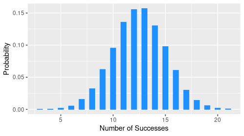
We can simulate a binomial distribution by tossing a coin n times. For each toss, if a head comes up, we’ll call it a success and map it to 1. Otherwise, it’s a failure and map it to 0. The probability of success is p. After n trials, we will count the number of successes. We will replicate this 10000 times and calculate the proportion of replications with k successes. Finally, we plot the resulting distribution. The code below is an implementation of this in R.

library(tidyverse)

n <- 25        # number of trials
p <- 0.5       # probability of success
reps <- 10000  # number of replications

num_success <- replicate(reps, {
  trials <- sample(c(0, 1), size = n, replace = TRUE, prob = c(1-p, p))
  sum(trials)
})

# Plot the number of success versus the proportion of replications
data.frame(num_success) %>%
  ggplot(aes(num_success)) +
  geom_bar(aes(y = ..prop..)) +
  labs(x = "Number of Successes", y = "Probability")