Basic Notions and Notation
Given an event \(A\), which is a subset of the sample space, i.e., \(A\subset\Omega\), we will associate with it a real number \(\mathbf{P}(A)\) to denote the probability that it will occur. The symbol \(\mathbf{P}\) is a probability distribution or probability measure.
Axioms
For \(\mathbf{P}\) to be a probability, it must satisfy these axioms:
-
non-negativity
\[\mathbf{P}(A)\geq0\] -
normalization
\[\mathbf{P}(\Omega)=1\] -
(finite) additivity
Given two events, \(A\) and \(B\), if \(A\cap B=\varnothing\), then
\[\mathbf{P}(A\cup B)=\mathbf{P}(A) + \mathbf{P}(B).\]We will strengthen this last axiom below.
Some Consequences of the Axioms
-
If \(A\cap B=\varnothing\), then
\[0\leq\mathbf{P}(A)\leq 1\] \[\mathbf{P}(\varnothing)=0\] \[\mathbf{P}(A\cup B)=\mathbf{P}(A)+\mathbf{P}(B).\] -
In general, if \(A_1, A_2,\ldots, A_k\) are disjoint, then
\[\mathbf{P}(A_1\cup\ldots\cup A_k)=\sum_{i=1}^{k}\mathbf{P}(A_i).\] -
If \(A\subset B\), then
\[\mathbf{P}(A)\leq\mathbf{P}(B).\] -
If \(A\cap B\neq\varnothing\), then
\[\mathbf{P}(A\cup B)=\mathbf{P}(A)+\mathbf{P}(B)-\mathbf{P}(A\cap B).\] -
Union Bound
\[\mathbf{P}(A\cup B)\leq\mathbf{P}(A)+\mathbf{P}(B)\]
Uniform Probability Law
Assume that the sample space \(\Omega\) consists of \(n\) equally likely elements and event \(A\) consists of \(k\) elements. Then,
\[\mathbf{P}(A)=\frac{k}{n}.\]Continuous Example
Consider all pairs \((x,y)\) such that \(0\leq x,y\leq 1\). We want to know the probability that \(x+y\leq\frac{1}{2}\). The plot below shows the sample space with the shaded region as the event of interest.
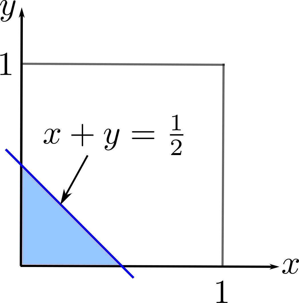
Therefore,
\[\mathbf{P}(\{x,y\,\vert\, x+y\leq\tfrac{1}{2}\})=\tfrac{1}{8}.\]This is just the area of the shaded region divided by the area of the square.
Discrete but Infinite Sample Space
Consider the sample space \(\{1,2,3,\ldots\}\). However, the elements are not equally likely with the probability given instead by
\[\mathbf{P}(n)=\frac{1}{2^n},\quad n=1,2,3,\ldots.\]The first axiom is obviously satisfied. To see that this satisfies the second axiom, we have
\[\mathbf{P}(\Omega)=\sum_{n=1}^{\infty}\frac{1}{2^n}=\frac{1}{2}\sum_{n=0}^{\infty}\frac{1}{2^n}=\frac{1}{2}\cdot\frac{1}{1-\tfrac{1}{2}}=1.\]Now, we want to know the probability of getting an even integer. We have
\[\begin{align} \mathbf{P}(\textbf{even})&=\mathbf{P}(\{2,4,6,\ldots\})\\ &=\mathbf{P}(\{2\}\cup\{4\}\cup\ldots) \end{align}\]Can we use the third axiom to continue our calculation? No. We have a union of infinitely many disjoint sets. To be able to continue, we need to introduce another axiom that will give us additivity for an infinite number of disjoint sets. This will be stated in the next section. For now, we proceed as if we can, i.e.,
\[\begin{align} \mathbf{P}(\textbf{even})&=\mathbf{P}(2)+\mathbf{P}(4)+\ldots\\ &=\frac{1}{2^2}+\frac{1}{2^4}+\ldots\\ &=\frac{1}{3}. \end{align}\]Countable Additivity Axiom
If \(A_1,A_2,A_3,\ldots\) is an infinite sequence of disjoint events, then
\[\mathbf{P}(A_1\cup A_2\cup A_3\cup\ldots)=\mathbf{P}(A_1)+\mathbf{P}(A_2)+\mathbf{P}(A_3)+\ldots\]Note that additivity holds only for countable sequences of events.
Bonferroni’s Inequality
For any events, \(A\) and \(B\),
\[\mathbf{P}(A\cap B)\geq\mathbf{P}(A)+\mathbf{P}(B)-1.\]In general, for \(n\) events \(A_1,\ldots,A_n\),
\[\mathbf{P}(A_1\cap\ldots\cap A_n)\geq\mathbf{P}(A_1)+\ldots+\mathbf{P}(A_n)-(n-1).\]