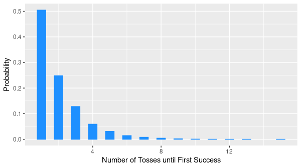
Geometric Distribution | The Science of Data

The geometric distribution represents the number of independent Bernoulli trials until the first success. For example, it describes the number of coin tosses needed to get a head, where head is considered as a success. It is a discrete probability distribution with one parameter $p$ and denoted by $\mathrm{Geom}(p)$.

Probability Mass Function

The probability mass function of a geometric distribution is given by

\[p_X(k)=(1-p)^{k-1}p\]

where $k=1,2,\ldots$

Expectation

The mean of a geometric distribution with parameter $p$ is

\[\mathbb{E}[X]=\dfrac{1}{p}.\]

Proof:

$$\begin{align} \mathbb{E}[X]&=\sum_{k=1}^{\infty}kp(1-p)^{k-1}\\ &=-p\,\dfrac{\mathrm{d}}{\mathrm{d}p}\sum_{k=1}^{\infty}(1-p)^k\\ &=-p\,\dfrac{\mathrm{d}}{\mathrm{d}p}\left[-1+\sum_{k=0}^{\infty}(1-p)^k\right]\\ &=-p\,\dfrac{\mathrm{d}}{\mathrm{d}p}\left(-1+\dfrac{1}{p}\right)\\ &=\frac{1}{p} \end{align}$$

Variance

The variance of a geometric random variable with parameter $p$ is

\[\mathrm{var}(X)=\dfrac{1-p}{p^2}.\]

Proof:

To begin, we have $$\begin{align} \mathrm{var}(X)&=\mathbb{E}[X^2]-(\mathbb{E}[X])^2\\ &=\sum_{k=1}^{\infty}k^2p(1-p)^{k-1}-\left(\frac{1}{p}\right)^2. \end{align}$$ Let's calculate the first term. $$\begin{align} \sum_{k=1}^{\infty}k^2p(1-p)^{k-1}&=-\sum_{k=1}^{\infty}kp\,\frac{\mathrm{d}}{\mathrm{d}p}(1-p)^k\\ &=-\sum_{k=1}^{\infty}kp\,\frac{\mathrm{d}}{\mathrm{d}p}\left[(1-p)^{k-1}(1-p)\right]\\ &=-\sum_{k=1}^{\infty}kp\!\left[(1-p)\frac{\mathrm{d}}{\mathrm{d}p}(1-p)^{k-1}-(1-p)^{k-1}\right]\\ &=-p(1-p)\frac{\mathrm{d}}{\mathrm{d}p}\sum_{k=1}^{\infty}k(1-p)^{k-1}+\sum_{k=1}^{\infty}kp(1-p)^{k-1}\\ &=p(1-p)\frac{\mathrm{d}^2}{\mathrm{d}p^2}\sum_{k=1}^{\infty}(1-p)^k+\mathbb{E}[X] \end{align}$$ Using the geometric series formula $$\sum_{k=0}^{\infty}x^k=\dfrac{1}{1-x}\qquad \text{for }|x|<1$$ we have $$\begin{align} \sum_{k=1}^{\infty}k^2p(1-p)^{k-1}&=p(1-p)\frac{\mathrm{d}^2}{\mathrm{d}p^2}\!\left[\dfrac{1}{1-(1-p)}-1\right]+\frac{1}{p}\\ &=p(1-p)\frac{\mathrm{d}^2}{\mathrm{d}p^2}\!\left(\frac{1}{p}-1\right)+\frac{1}{p}\\ &=p(1-p)\!\left(\frac{2}{p^3}\right)+\frac{1}{p}\\ &=\frac{2(1-p)}{p^2}+\frac{1}{p}\\ &=\frac{2-p}{p^2}. \end{align}$$ Finally, $$\begin{align} \mathrm{var}(X)&=\frac{2-p}{p^2}-\frac{1}{p^2}\\ &=\frac{1-p}{p^2}. \end{align}$$

Conditioning

Suppose now that the first trial was a failure. What is the distribution of the remaining trials until the first success? Because we are dealing with independent trials, the remaining trials will still have a geometric distribution, i.e., conditioned on $X>1$, $X-1$ is geometric with parameter $p$.

Memorylessness

In general, if the first $n$ trials are failures, then the remaining trials will still be geometric, i.e., conditioned on $X>n$, $X-n$ is geometric with parameter $p$. This property is called memorylessness.

Note:

Another way of deriving the variance of a geometric random variable is by using its memorylessness property.

Monte Carlo Simulation

library(tidyverse)

reps <- 10000 # number of replications
p <- 0.5      # probability of success

# Initialize vector for the replications
tosses_to_success <- 0

for (i in 1:reps) {
  success <- 0
  counter <- 0
  while (success == 0) {
    counter <- counter + 1
    toss <- sample(c(0, 1), size = 1, replace = TRUE, prob = c(1-p, p))
    success <- success + toss
  }
  tosses_to_success[i] <- counter
}

# Plot the distribution
data.frame(tosses_to_success) %>%
  ggplot(aes(tosses_to_success, y = ..prop..)) +
  geom_bar() +
  labs(x = "Number of Tosses Until First Success", y = "Probability")