The hypergeometric distribution is a discrete random variable with three parameters: the population size \(n\), the event count \(r\), and the sample size \(m\). It describes the probability of getting \(k\) items of interest when sampling \(m\) items, without replacement, from a population of \(n\) that includes \(r\) items of interest.
Hypergeometric versus Binomial Distributions
The key difference between the hypergeometric and the binomial distributions is the sampling method. In the hypergeometric case, we are sampling without replacement so that the trials are dependent, i.e., the outcome of a trial affects the outcome of the following trials. In the binomial case, they are independent because we are sampling with replacement. To illustrate this, consider a bowl with 7 black and 3 white marbles. For the first trial, the probability of picking a black marble is \(\tfrac{7}{10}\). If we picked a black marble and did not replace it, the probability of picking another black marble in the second trial will be \(\tfrac{6}{9}\). However, if we replaced it, then the probability of getting a black marble the second time will still be \(\tfrac{7}{10}\).
Probability Mass Function
The probability mass function for a hypergeometric distribution is
\[p_X(k)=\dfrac{\displaystyle\binom{r}{k}\binom{n-r}{m-k}}{\displaystyle\binom{n}{m}}.\]Expectation
The mean of a hypergeometric distribution is
\[\mathbb{E}[X]=\frac{mr}{n}.\]We begin with $$\mathbb{E}[X]=\sum_{k}kp_X(k)=\sum_{k}k\,\dfrac{\binom{r}{k}\binom{n-r}{m-k}}{\binom{n}{m}}.$$ Note that $$k\binom{r}{k}=\frac{r!}{(k-1)!(r-k)!}=\frac{r(r-1)!}{(k-1)!(r-1-(k-1))!}=r\binom{r-1}{k-1}$$ and $$\binom{n}{m}=\frac{n!}{m!(n-m)!}=\frac{n(n-1)!}{m(m-1)!(n-1-(m-1))!}=\frac{n}{m}\binom{n-1}{m-1}.$$ Hence, $$\begin{align} \mathbb{E}[X]&=\frac{mr}{n}\sum_{k}\dfrac{\binom{r-1}{k-1}\binom{(n-1)-(r-1)}{(m-1)-(k-1)}}{\binom{n-1}{m-1}}\\ &=\frac{mr}{n} \end{align}$$ where the summed term is another hypergeometric PMF and we used the normalization condition $$\sum_{k}\dfrac{\binom{r}{k}\binom{n-r}{m-k}}{\binom{n}{m}}=1.$$
Variance
The variance of a hypergeometric random variable is
\[\mathrm{var}(X)=\frac{mr(n-r)(n-m)}{n^2(n-1)}.\]To calculate the variance, we have to do a bit more maneuvering. We start by noting that $$\frac{\binom{r}{k}\binom{n-r}{m-k}}{\binom{n}{m}}=\frac{r(r-1)}{k(k-1)}\frac{m(m-1)}{n(n-1)}\dfrac{\binom{r-2}{k-2}\binom{(n-2)-(r-2)}{(m-2)-(k-2)}}{\binom{n-2}{m-2}}.$$ We can massage the formula for variance to get $$\begin{align} \mathrm{var}(X)&=\mathbb{E}[X^2]-(\mathbb{E}[X])^2\\ &=\mathbb{E}[X(X-1)]+\mathbb{E}[X]-(\mathbb{E}[X])^2\\ &=\mathbb{E}[X(X-1)]+\mathbb{E}[X](1-\mathbb{E}[X]). \end{align}$$ The first term is $$\begin{align} \mathbb{E}[X(X-1)]&=\sum_{k}k(k-1)p_X(k)\\ &=\dfrac{r(r-1)m(m-1)}{n(n-1)}\sum_{k}\dfrac{\binom{r-2}{k-2}\binom{(n-2)-(r-2)}{(m-2)-(k-2)}}{\binom{n-2}{m-2}}\\ &=\dfrac{mr(r-1)(m-1)}{n(n-1)}. \end{align}$$ Hence, $$\begin{align} \mathrm{var}(X)&=\dfrac{mr(r-1)(m-1)}{n(n-1)}+\frac{mr}{n}\left(1-\frac{mr}{n}\right)\\ &=\frac{mr}{n}\left[\frac{(r-1)(m-1)}{n-1}+1-\frac{mr}{n}\right]\\ &=\frac{mr}{n}\left[\dfrac{n(r-1)(m-1)+(n-1)(n-mr)}{n(n-1)}\right]\\ &=\frac{mr}{n}\left[\dfrac{mrn-rn-mn+n+n^2-n-mrn+mr}{n(n-1)}\right]\\ &=\frac{mr}{n}\frac{n(n-m)-r(n-m)}{n(n-1)}\\ &=\frac{mr(n-r)(n-m)}{n^2(n-1)}. \end{align}$$
Monte Carlo Simulation
library(tidyverse)
# Set the parameters
n <- 500 # Number of items in the bowl
r <- 100 # Number of red items in the bowl
m <- 50 # Number of items to pick
# Create a bowl with n items, r are red
# Identify 1 as red and 0 otherwise
bowl <- sample(rep(c(0,1), c(n-r,r)))
B <- 10000 # Number of replications
# Pick m items from bowl and replicate B times
trials <- replicate(B, {
items_picked <- sample(bowl, m, replace = FALSE)
sum(items_picked)
})
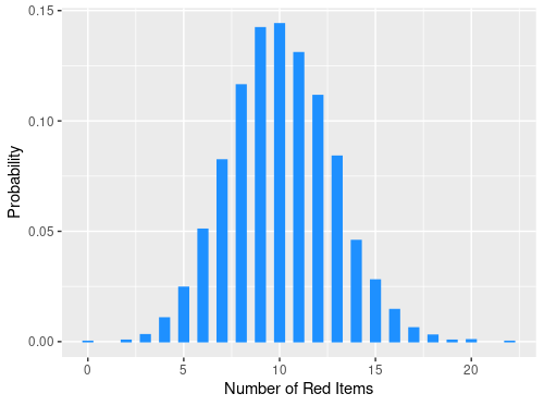
# Plot the distribution
data.frame(trials) %>%
ggplot(aes(trials, y=..prop..)) +
geom_bar(width = 0.5, color = "dodgerblue", fill = "dodgerblue") +
labs(x = "Number of Red Items", y = "Probability")