The negative binomial distribution is a generalization of the geometric distribution. It represents the number of independent Bernoulli trials \(k\) until \(r\) successes is achieved. It is described by two parameters, the stopping parameter \(r\) and the probability of success \(p\).
Probability Mass Function
Any sequence of \(k\) Bernoulli trials with \(r\) successes can occur with probability
\[p^r(1-p)^{k-r}.\]Because the last trial is always a success, we can distribute the remaining \(r-1\) successes to the \(k-1\) trials in \(\binom{k-1}{r-1}\) ways. Therefore, the PMF for a negative binomal random variable is
\[p_X(k)=\binom{k-1}{r-1}p^r(1-p)^{k-r}\]where \(k=r,r+1,\ldots\)
A negative binomial random variable is also the sum of \(r\) independent geometric random variables with parameter \(p\), i.e.,
\[X=X_1+\ldots+X_r\]where \(X_i\sim\mathrm{Geom}(p).\)
Expectation
The expectation of a negative binomial distribution is
\[\mathbb{E}[X]=\frac{r}{p}.\]$$\begin{align} \mathbb{E}[X]&=\mathbb{E}[X_1]+\ldots+\mathbb{E}[X_r]\\ &=\frac{1}{p}+\ldots+\frac{1}{p}\\ &=\frac{r}{p} \end{align}$$
Variance
The variance of a negative binomial distribution is
\[\mathrm{var}(X)=\dfrac{r(1-p)}{p^2}.\]$$\begin{align} \mathrm{var}(X)&=\mathrm{var}(X_1)+\ldots+\mathrm{var}(X_r)\\ &=\frac{1-p}{p^2}+\ldots+\frac{1-p}{p^2}\\ &=\dfrac{r(1-p)}{p^2}. \end{align}$$
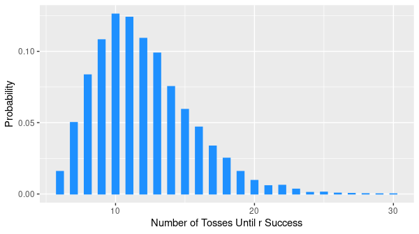
Monte Carlo Simulation
library(tidyverse)

reps <- 10000 # number of replications

r <- 6    # number of successes
p <- 0.5  # probability of a success

# Initialize vector for the replications
tosses_to_r_success <- 0

for (i in 1:reps) {
  successes <- 0
  counter <- 0
  while (successes != r) {
    counter <- counter + 1
    toss <- sample(c(0, 1), size = 1, replace = TRUE, prob = c(1-p, p))
    successes <- successes + toss
  }
  tosses_to_r_success[i] <- counter
}

# Plot the distribution
data.frame(tosses_to_r_success) %>%
  ggplot(aes(tosses_to_r_success, y = ..prop..)) +
  geom_bar() +
  labs(x = "Number of Tosses Until r Successes", y = "Probability")